KalsusEvening/Melbourne_Housing_Regression

Melbourne Housing Price Prediction

📹 Video Presentation

(https://youtu.be/N3SE29PIr7g)

---

📋 Project Overview

This project builds a complete machine learning pipeline to predict Melbourne housing prices using both regression (exact price) and classification (price category) models.

Dataset	Melbourne Housing Snapshot (Kaggle)
Original Size	13,580 properties, 21 features
Final Size	11,139 properties (82% retained)
Target	Price

Goals

1. Build baseline regression model and improve through feature engineering
2. Apply K-Means clustering to discover property segments
3. Convert to classification and train classification models
4. Compare models and identify best performers

---

📊 Part 1-2: Exploratory Data Analysis

Data Cleaning Summary

Step	Action	Impact
Missing Values	Dropped BuildingArea (47% missing), YearBuilt (40% missing)	-
Imputation	Car (median), CouncilArea (mode)	~1,200 rows
Outliers	Removed using IQR method	2,441 rows
Final	11,139 rows retained	18% removed

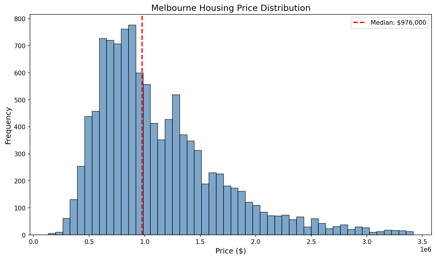
Price Distribution

Statistics: Mean $1.12M | Median $976K | Range $131K - $3.42M

---

Research Question 1: Property Type vs Price

Type	Count	Mean Price
House	9,055 (81%)	$1,203,259
Townhouse	952 (9%)	$936,054
Unit	1,132 (10%)	$640,529

Finding: Houses cost $560K more than units on average.

---

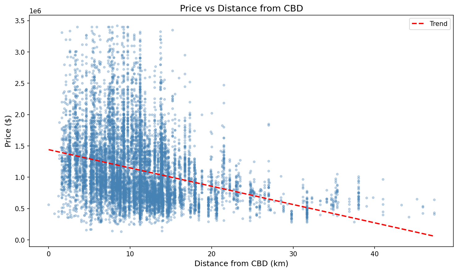
Research Question 2: Distance from CBD

Distance	Avg Price
0-5 km	$1,361K
10-15 km	$1,046K
30+ km	$597K

Finding: Every 5km from CBD reduces price by ~$100-150K. Correlation: -0.31

---

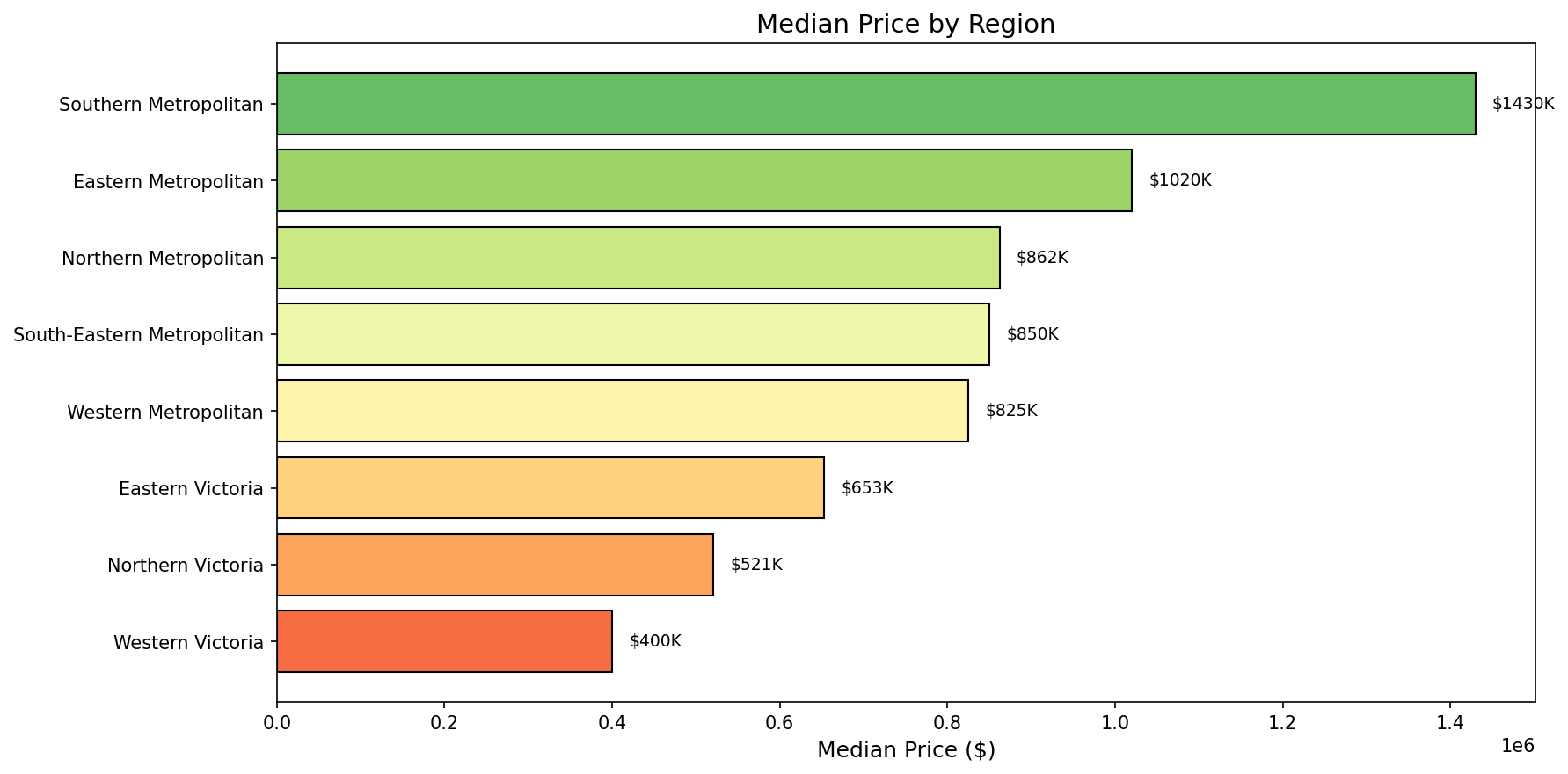
Research Question 3: Regional Price Differences

Finding: Southern Metropolitan commands 3.5× premium over Western Victoria.

---

Correlation Analysis

Top Correlations with Price:

• Rooms: +0.41
• Bathroom: +0.40
• Distance: -0.31

---

📈 Part 3: Baseline Model

Metric	Value
Algorithm	Linear Regression
Features	7 numeric
R² Score	0.4048
MAE	$323,527
RMSE	$425,453

Interpretation: Model explains only 40% of price variance. Significant room for improvement through feature engineering.

---

🔧 Part 4: Feature Engineering

Features Expanded: 7 → 43

Category	Features	Count
Original Numeric	Rooms, Distance, Bathroom, etc.	7
One-Hot Encoded	Type, Method, Regionname	16
Derived Features	Ratios, indicators, bins	7
Cluster Features	Labels + distances to centroids	8
Total		43

New Derived Features

Feature	Purpose
Rooms_per_Bathroom	Property efficiency
Total_Spaces	Overall size indicator
Land_per_Room	Land generosity
Is_Inner_City	Location premium flag
Luxury_Score	Amenity indicator

---

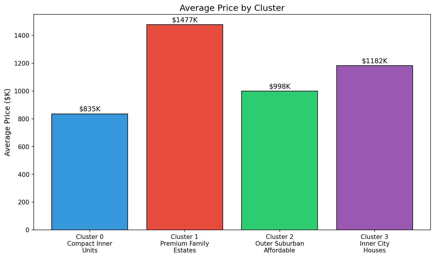
K-Means Clustering (k=4)

We used the Elbow Method and Silhouette Score to determine k=4 clusters.

Cluster	Profile	Avg Price	Avg Distance	Avg Rooms
0	Compact Inner Units	$835K	8.0 km	2.0
1	Premium Family Estates	$1.48M	12.9 km	4.2
2	Outer Suburban Affordable	$998K	13.7 km	3.0
3	Inner City Houses	$1.18M	7.9 km	3.1

Key Insight: Two distinct pricing drivers discovered:

• Location premium (Clusters 0 & 3): Close to CBD
• Size premium (Clusters 1 & 2): Larger properties

---

🎯 Part 5: Improved Regression Models

Model	R² Score	MAE	Improvement
Baseline Linear Reg	0.4048	$323,527	-
Improved Linear Reg	0.6302	$244,654	+55.7%
Random Forest	0.7752	$178,455	+91.5%
Gradient Boosting	0.7900	$172,891	+95.1%

Feature Importance (Random Forest)

Top 5 Most Important Features:

Rank	Feature	Importance
1	Regionname_Southern Metropolitan	0.242
2	Distance	0.172
3	Type_h (House)	0.137
4	Dist_to_Cluster_0	0.099
5	Landsize	0.062

Key Insights:

• Location dominates (Region + Distance)
• Clustering features in top 15 (validated approach)
• Engineered features proved valuable

---

🏆 Part 6: Regression Winner

Gradient Boosting Regressor

Metric	Value
R² Score	0.7900
MAE	$172,891
RMSE	$252,728
Improvement over Baseline	+95.1%

Why Gradient Boosting Won:

• Captures non-linear relationships
• Sequential learning corrects errors iteratively
• Best balance of accuracy and generalization

Saved as: regression_model_gradient_boosting.pkl

---

🔄 Part 7: Regression to Classification

We converted continuous Price into 3 balanced categories using quantile binning:

Class	Price Range	Count	Percentage
Low	< $800,000	3,593	32.3%
Medium	$800K - $1.24M	3,759	33.7%
High	> $1.24M	3,787	34.0%

Balance: Imbalance ratio of 1.05 - classes are well balanced.

---

Precision vs Recall Analysis

For housing price prediction, Precision is more important:

Error Type	Meaning	Consequence
False Positive	Predict High, actually Low	Buyer overpays significantly
False Negative	Predict Low, actually High	Seller underprices

Conclusion: False Positives are worse for buyers - prioritize Precision.

---

📊 Part 8: Classification Models

Model	Accuracy
Logistic Regression	71.1%
Random Forest	77.1%
Gradient Boosting	78.9%

Winner Performance: Gradient Boosting Classifier

Class	Precision	Recall	F1-Score
Low	0.85	0.86	0.85
Medium	0.69	0.70	0.70
High	0.83	0.81	0.82

Observations:

• Medium class hardest to predict (borders both Low and High)
• High precision for High class (0.83) - reliable for buyers
• Gradient Boosting wins both regression AND classification

Saved as: classification_model_gradient_boosting.pkl

---

📁 Repository Files

File	Description	Size
regression_model_gradient_boosting.pkl	Regression model (R²=0.79)	419 KB
classification_model_gradient_boosting.pkl	Classification model (78.9%)	1.15 MB
scaler.pkl	Regression StandardScaler	2.32 KB
classification_scaler.pkl	Classification StandardScaler	2.32 KB
feature_names.pkl	43 feature names	762 B
Assignment_2_....ipynb	Complete Jupyter notebook	6.48 MB

---

💡 Key Takeaways

What Worked Well

1. Feature engineering was crucial - Linear Regression R² improved from 0.40 to 0.63 (+55%)
2. Clustering added value - 4 cluster features in top 15 importance
3. Ensemble methods excel - Gradient Boosting won both tasks
4. Location is paramount - Region and distance dominate predictions

Challenges

1. Medium price class hardest to predict (boundary cases)
2. Multicollinearity between Rooms and Bedroom2 (0.94 correlation)
3. Right-skewed price distribution required careful outlier handling

Lessons Learned

1. Always establish a baseline before feature engineering
2. EDA guides modeling decisions
3. Clustering reveals hidden patterns
4. Same algorithm can perform dramatically different with good features

---

📊 Final Summary

Task	Baseline	Final Model	Improvement
Regression R²	0.4048	0.7900	+95.1%
Regression MAE	$323,527	$172,891	-46.6%
Classification Accuracy	-	78.9%	-
Features Used	7	43	+36

---

---

🤖 Tools & Methodology

Use of AI Assistance

This project was completed with the assistance of Claude (Anthropic) as a coding and learning partner.

Why I used Claude:

• To understand best practices for structuring a machine learning pipeline
• To learn proper implementation of sklearn models and evaluation metrics
• To get explanations of concepts like feature engineering, clustering, and model evaluation
• To debug code and understand error messages
• To ensure consistent documentation and code commenting

What I learned through this process:

• The importance of establishing baselines before optimization
• How feature engineering can dramatically improve model performance
• The difference between regression and classification evaluation metrics
• How to interpret clustering results and use them as features
• Best practices for presenting data science work

All code was executed, tested, and validated by me in Google Colab. The final analysis, interpretations, and conclusions are my own understanding of the results.

---

👤 Author

David Wilfand

Assignment #2: Classification, Regression, Clustering, Evaluation

---

📚 References

• Dataset: Melbourne Housing Snapshot - Kaggle
• Tools: scikit-learn, pandas, numpy, matplotlib, seaborn
• Algorithms: Linear Regression, Random Forest, Gradient Boosting, K-Means